Section outline
-

-
Hello, everyone!
In this course portal, we’re excited to talk to you about something incredibly fascinating and powerful in the world of mathematics: numerical methods.
Numerical methods are powerful tools that solve complex problems in science, engineering, and daily life. Whether you’re calculating the weather forecast or simulating the dynamics of a car engine, numerical methods are at work.
-
After completing this topic, you will be able to
- state the definition of numerical methods. (Section 1.1)
- compare between analytical solutions and numerical solutions. (Section 1.2)
- identify the advantages and disadvantages of numerical methods. (Section 1.3)
Estimated student learning time: 2 hours -
Please watch the following Webex Video (07:00) before you start to learn about this course. In this video, I briefly explain the structure of the course content on PEARL.
-
FileView
-
-
There are 3 subtopics for this course. Study all the given learning materials before proceeding to the next section which discuss some examples of numerical methods.
-
We begin our lesson with the definition of "Numerical Methods".
-
From the definition of numerical method, we know that approximate solution is the type of solution that obtained by using numerical method while the exact or analytical solution is the true solution.
Let's watch the following Lecture Recording 1.2 (06:38) which discuss the comparison between exact solution and approximation. The PowerPoint slides 1.2 are also attached.
-
View
-
View
-
-
Why Do We Need Numerical Methods?
Drawback of Numerical Methods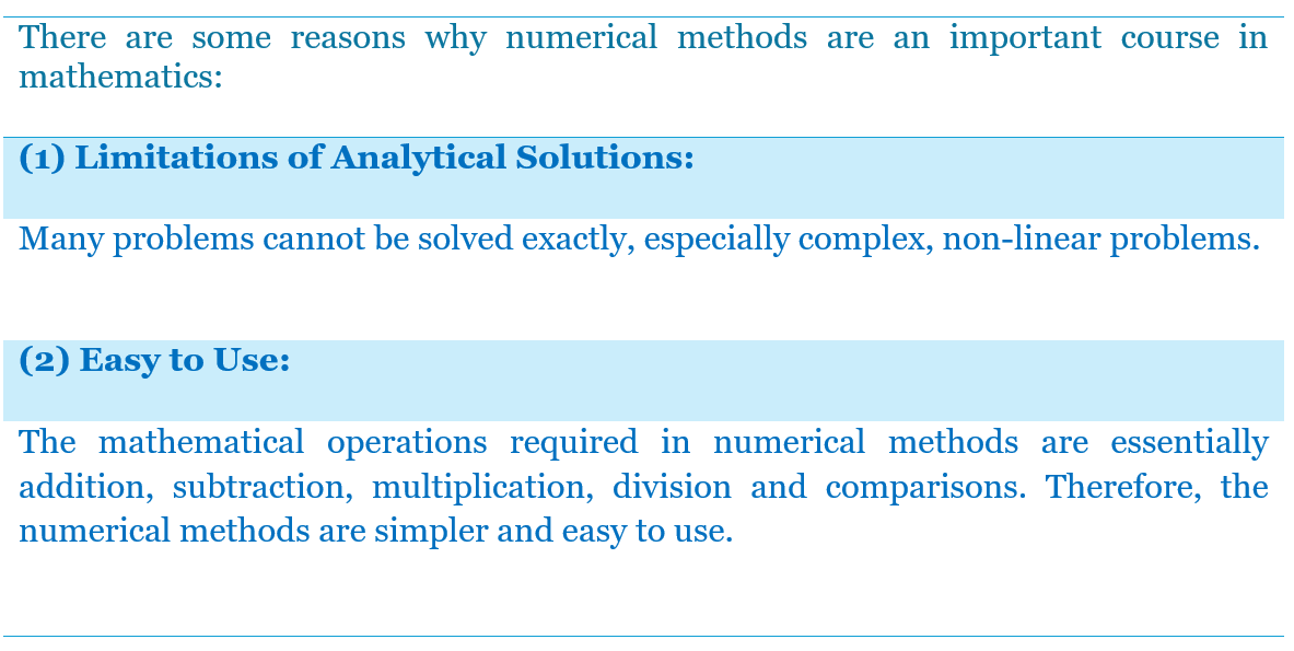
Numerical methods have also limitations when solving a problem.
- The solution is not exact but only approximate solutions.
- Besides, it is necessary to provide initial estimates of the unknowns in the beginning of the step.
- The process of obtaining the solution using numerical methods normally involves large number of tedious arithmetic calculations. *
* However, “tedious arithmetic calculation” is not a problem anymore with the development of fast and efficient computers.
* There are many commercial and user-friendly numerical software packages, such as NAG) Library, Mathematica, MATLAB, Python (NumPy), R, etc., one can write the numerical method algorithm or simply use the “canned” functions or functions in software libraries to solve the complicated problems.
-
Let's spend some time to think about the following scenario:
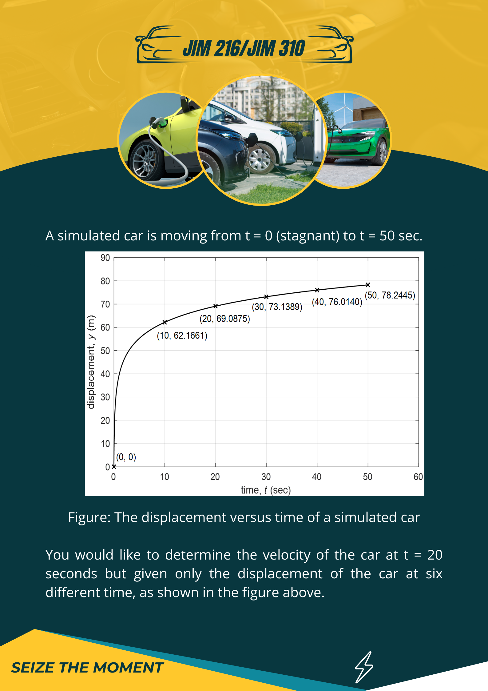
To answer the question in the figure above, you recall the formula of velocity

where
 = velocity,
  =displacement,
  = time.
But in the figure above, the values of y are given instead of function of y.
You might be thinking, we cannot determine
 because the function
 ") is
not given.
is
not given.“YES, you are right!”
We have only values of displacements at certain time intervals when observed from the figure, but the function of displacement which in terms of time is not provided, hence we cannot determine
 .
.HOWEVER, we may still solve this kind of question using a technique called Numerical Differentiation in Numerical Methods.
For example, by using forward-difference formula with accuracy
") (note that this formula is also called as three-point endpoint
formula):
(note that this formula is also called as three-point endpoint
formula): \approx \frac{-3 f(x_0)+4 f(x_0+h)-f(x_0+2h)}{2h}")
We obtain the velocity of the car at
 20 seconds as below:
 \approx \frac{-3 y(20)+4 y(30)-y(40)}{2(10)}")
 \approx \frac{-3(69.0875)+4(73.1389)-(76.0140)}{20}=") 0.4640 ms-1
0.4640 ms-1
-
There are two examples of Numerical Methods that will be discussed.
Example 1:
Here, we introduce another fundamental numerical method which is called Newton-Raphson method, or simply called Newton’s method. This method is able to determine the root of equation quickly and efficiently especially for the complex equation where traditional algebra falls short.
Watch the following YouTube video (07:21) from the channel “MathAndPhysics”.
(P/s: If there is an error to load the video from this platform, please click "Watch on YouTube".
From the video at 00:34, the blue colour solid curve is the graph of a function
") . We want to determine the root of equation
. We want to determine the root of equation =0") . It is the intersection of the curve with the
. It is the intersection of the curve with the  axis,
axis,  .
. Let say we do not know this true solution. The red dot
 (at 00:45) is the initial guess of solution.
 You will see that from this initial guess we will develop a new green colour tangent line (at 00:56). This tangent line intersects the
axis at approximately  .
. Hence, the approximate solution has improved from
to . Now is denoted as a new red dot, represents the second guess of the solution. Repeat the same procedures, the intersection point becomes closer and closer to the true solution.
Note: You may stop the video after 2:09 as our intension here is not teaching you the formula of the Newton-Raphson method, but rather to show you how Newton-Raphson method iterates and converges to the true solution.
Next, we see another example which demonstrates the powerful of numerical methods in solving an integration problem.
Example 2:
We use the formula that learned in Calculus to determine the area under a curve. This topic is called analytical integration, and the result we obtain is an analytical solution. On the other hand, in numerical methods, there is a topic named numerical integration. As expected, the solution obtained by numerical integration is only an approximation.
Watch the following YouTube video (02:36) by StudySession channel.
This video explains and compares between the analytical integration and numerical integration. You will see that for numerical integration, the area under the curve is divided into sub-intervals, then approximate the area of each block is equivalent to the area of rectangles. Hence, the integration of the function is the sum of the areas of all rectangles.
From Example 1 and Example 2 , you will notice that the concept of numerical methods is easy and straightforward. These numerical methods can be used to solve complex mathematical problems easily using iterative methods.
-
There are many applications of numerical methods in various fields:
- Engineering: Imagine designing a skyscraper. Engineers use numerical methods to simulate how the structure will respond to various forces and ensure it’s safe and sound.
- Finance: In the stock market, numerical methods help predict price movements and manage financial risks.
- Medicine: Doctors use numerical simulations to understand how diseases progress and how treatments affect the human body.
- Climate: Meteorologists rely on numerical models to predict the weather and study climate change.
To gain more ideas, please click the following link which connected to an article about Real-Life Applications of Numerical Analysis in the platform GeeksforGeeks:
Real-Life Applications of Numerical Analysis - GeeksforGeeks
-
Go to the Website of Holistic Numerical Methods:
https://nm.mathforcollege.com/chapter-3-bisection-method/
This course was developed by the University of South Florida, funded partially by the National Science Foundation under Grant Number 2013271.
This chapter is about the bisection method that is commonly used to solve nonlinear equation. Click into the simulation which shows the GUI (graphical user interface) as below:
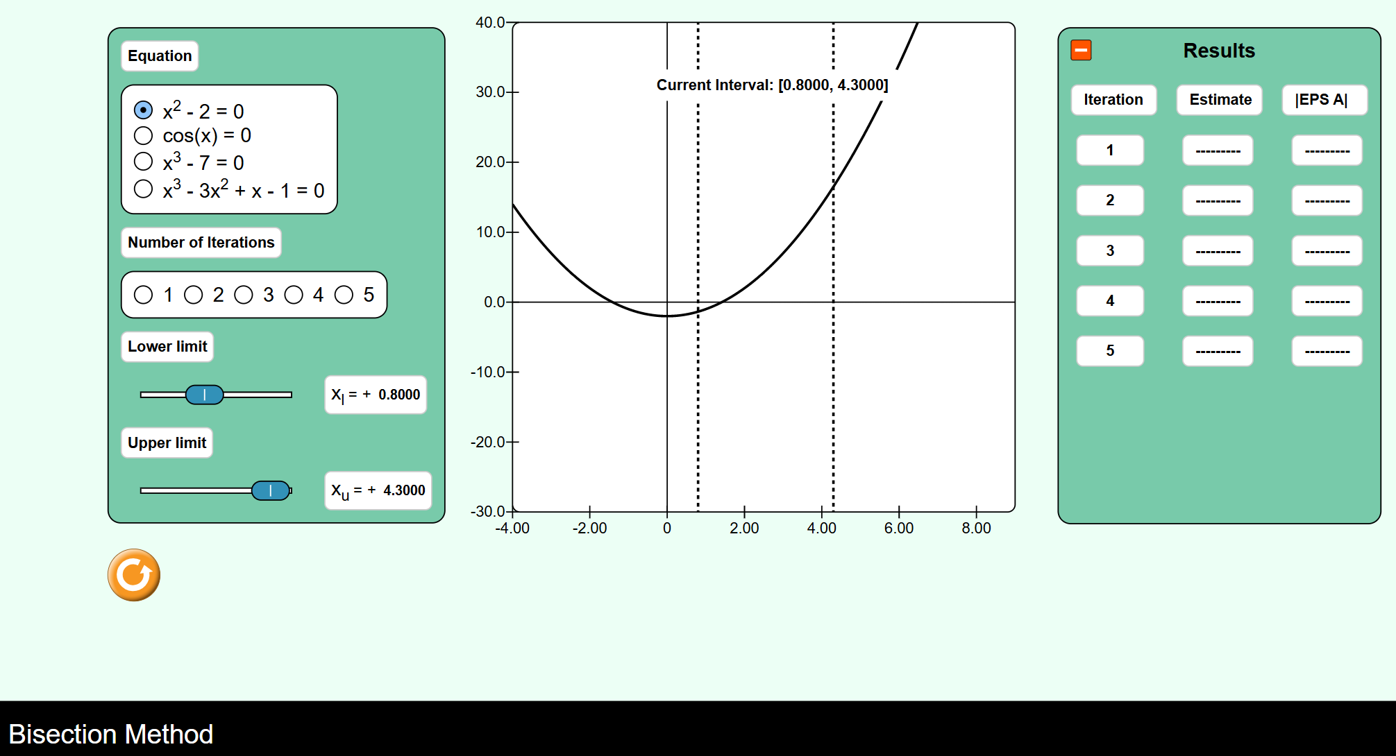
There are four nonlinear equations in the simulation.
- Explore each of the equation to see how the solution converges by clicking the number of iterations.
- You may set different lower and upper limits. Make sure that the limits interval that you set must bracketing the solution, i.e. the x-intersection points.
-
Complete the quiz below. The estimated time to finish is 10 minutes. You can retake the quiz as many times as you'd like, and the system will record your highest score.
-
QuizView Make attempts: 1 Receive a grade
-
-
Watch the promotional video (03:58) by Professor Jeffrey Chasnov who is the mathematics professor at Hong Kong University.
Prof. Chasnov introduces the course “Numerical Methods for Engineers”, highlights the capability of numerical methods in solving various engineering problems such as
- Mechanical and aerospace engineering (computational fluid dynamics),
- Geoengineering (climate change and global warming),
- Bioengineering (immunology, cell biology and genomics)
- Chemical engineering (computational chemistry in developing new drugs)
- Computer engineering and data science (machine learning)
-
We have seen that numerical methods are essential in bridging the gap between theoretical mathematics and practical applications. If you are excited to dive deeper, our undergraduate mathematics program offers many opportunities to explore and master these techniques.
-
-
GlossaryView Make entries: 1
-
-
- Burden, R.L. and Faires, J.D. (2015). Numerical Analysis. 10th Edition. California: Brooks/Cole, Cengage Learning.
- Chapra, S.C. and Canale R.P. (2020). Numerical Methods for Engineers. 8th International Edition. New York: McGraw-Hill.